Extracting meaningful features¶

You may notice that the name nilearn is reminiscent of scikit-learn, a popular Python library for machine learning. This is no accident! Nilearn and scikit-learn were created by the same team, and nilearn is designed to bring machine LEARNing to the NeuroImaging (NI) domain.

With that in mind, let’s briefly consider why we might want specialized tools for working with neuroimaging data. When performing a machine learning analysis, our data often look something like this:

from sklearn import datasets

# This will return a 'Bunch' object
# see sklearn.utils.Bunch for details
diabetes = datasets.load_diabetes(as_frame=True)

# We can return information on the dataset
print(diabetes.DESCR)

# And view its contents
diabetes.data.head()

.. _diabetes_dataset:

Diabetes dataset
----------------

Ten baseline variables, age, sex, body mass index, average blood
pressure, and six blood serum measurements were obtained for each of n =
442 diabetes patients, as well as the response of interest, a
quantitative measure of disease progression one year after baseline.

**Data Set Characteristics:**

  :Number of Instances: 442

  :Number of Attributes: First 10 columns are numeric predictive values

  :Target: Column 11 is a quantitative measure of disease progression one year after baseline

  :Attribute Information:
      - age     age in years
      - sex
      - bmi     body mass index
      - bp      average blood pressure
      - s1      tc, total serum cholesterol
      - s2      ldl, low-density lipoproteins
      - s3      hdl, high-density lipoproteins
      - s4      tch, total cholesterol / HDL
      - s5      ltg, possibly log of serum triglycerides level
      - s6      glu, blood sugar level

Note: Each of these 10 feature variables have been mean centered and scaled by the standard deviation times `n_samples` (i.e. the sum of squares of each column totals 1).

Source URL:
https://www4.stat.ncsu.edu/~boos/var.select/diabetes.html

For more information see:
Bradley Efron, Trevor Hastie, Iain Johnstone and Robert Tibshirani (2004) "Least Angle Regression," Annals of Statistics (with discussion), 407-499.
(https://web.stanford.edu/~hastie/Papers/LARS/LeastAngle_2002.pdf)

	age	sex	bmi	bp	s1	s2	s3	s4	s5	s6
0	0.038076	0.050680	0.061696	0.021872	-0.044223	-0.034821	-0.043401	-0.002592	0.019908	-0.017646
1	-0.001882	-0.044642	-0.051474	-0.026328	-0.008449	-0.019163	0.074412	-0.039493	-0.068330	-0.092204
2	0.085299	0.050680	0.044451	-0.005671	-0.045599	-0.034194	-0.032356	-0.002592	0.002864	-0.025930
3	-0.089063	-0.044642	-0.011595	-0.036656	0.012191	0.024991	-0.036038	0.034309	0.022692	-0.009362
4	0.005383	-0.044642	-0.036385	0.021872	0.003935	0.015596	0.008142	-0.002592	-0.031991	-0.046641

For our purposes, what’s most interesting is the structure of this data set. That is, the data is structured in a tabular format, with pre-extracted features of interest. This makes it easier to consider issues such as: which features would we like to predict? Or, how should we handle cross-validation?

But if we’re starting with neuroimaging data, how can create this kind of structured representation? In this tutorial, we’ll use our sample neuroimaging data and a pre-defined functional atlas to derive connectomes that we can use in our subsequent classification analyses. While your extracted features of interest may differ depending on your downstream analyses (e.g., you may want to use a different atlas), this basic structure is useful for a range of research questions!

Neuroimaging data¶

Neuroimaging data does not have a tabular structure. Instead, it has both spatial and temporal dependencies between successive data points. That is, knowing where and when something was measured tells you information about the surrounding data points.

We also know that neuroimaging data contains a lot of noise that’s not blood-oxygen-level dependent (BOLD), such as head motion. Since we don’t think that these other noise sources are related to neuronal firing, we need to consider how we can make sure that our analyses are not driven by these noise sources.

These are all considerations that most machine learning software libraries are not designed to deal with! Nilearn therefore plays a crucial role in bringing machine learning concepts to the neuroimaging domain.

To get a sense of the problem, the quickest method is to just look at some data. You may have your own data locally that you’d like to work with. Nilearn also provides access to several neuroimaging data sets and atlases (we’ll talk about these a bit later).

These data sets (and atlases) are only accessible because research groups chose to make their collected data publicly available. We owe them a huge thank you for this! The data set we’ll use today was originally collected by Rebecca Saxe’s group at MIT and is hosted on OpenNeuro.

The nilearn team preprocessed the data set with fMRIPrep and downsampled it to a lower resolution, so it’d be easier to work with. We can learn a lot about this data set directly from the Nilearn documentation. For example, we can see that this data set contains over 150 children and adults watching a short Pixar film. Let’s download just the first 30 participants.

from nilearn import datasets

development_dataset = datasets.fetch_development_fmri(n_subjects=30)

Dataset created in /home/runner/nilearn_data/development_fmri

Dataset created in /home/runner/nilearn_data/development_fmri/development_fmri

Downloading data from https://osf.io/yr3av/download ...

 ...done. (2 seconds, 0 min)

Downloading data from https://osf.io/download/5c8ff3df4712b400183b7092/ ...

 ...done. (1 seconds, 0 min)

Downloading data from https://osf.io/download/5c8ff3e04712b400193b5bdf/ ...

 ...done. (1 seconds, 0 min)

Downloading data from https://osf.io/download/5c8ff3e14712b400183b7097/ ...

 ...done. (1 seconds, 0 min)

Downloading data from https://osf.io/download/5c8ff3e32286e80018c3e42c/ ...

 ...done. (1 seconds, 0 min)

Downloading data from https://osf.io/download/5c8ff3e4a743a9001760814f/ ...

 ...done. (1 seconds, 0 min)

Downloading data from https://osf.io/download/5c8ff3e54712b400183b70a5/ ...

 ...done. (1 seconds, 0 min)

Downloading data from https://osf.io/download/5c8ff3e52286e80018c3e439/ ...

 ...done. (2 seconds, 0 min)

Downloading data from https://osf.io/download/5c8ff3e72286e80017c41b3d/ ...

 ...done. (1 seconds, 0 min)

Downloading data from https://osf.io/download/5c8ff3e9a743a90017608158/ ...

 ...done. (1 seconds, 0 min)

Downloading data from https://osf.io/download/5c8ff3e82286e80018c3e443/ ...

 ...done. (2 seconds, 0 min)

Downloading data from https://osf.io/download/5c8ff3ea4712b400183b70b7/ ...

 ...done. (1 seconds, 0 min)

Downloading data from https://osf.io/download/5c8ff3eb2286e80019c3c194/ ...

 ...done. (1 seconds, 0 min)

Downloading data from https://osf.io/download/5c8ff37da743a90018606df1/ ...

 ...done. (2 seconds, 0 min)

Downloading data from https://osf.io/download/5c8ff37c2286e80019c3c102/ ...

 ...done. (1 seconds, 0 min)

Downloading data from https://osf.io/download/5cb4701e3992690018133d4f/ ...

 ...done. (2 seconds, 0 min)

Downloading data from https://osf.io/download/5cb46e6b353c58001b9cb34f/ ...

 ...done. (1 seconds, 0 min)

Downloading data from https://osf.io/download/5c8ff37d4712b400193b5b54/ ...

 ...done. (1 seconds, 0 min)

Downloading data from https://osf.io/download/5c8ff37d4712b400183b7011/ ...

 ...done. (1 seconds, 0 min)

Downloading data from https://osf.io/download/5c8ff37e2286e80016c3c2cb/ ...

 ...done. (1 seconds, 0 min)

Downloading data from https://osf.io/download/5c8ff3832286e80019c3c10f/ ...

 ...done. (1 seconds, 0 min)

Downloading data from https://osf.io/download/5c8ff3822286e80018c3e37b/ ...

 ...done. (1 seconds, 0 min)

Downloading data from https://osf.io/download/5c8ff382a743a90018606df8/ ...

 ...done. (1 seconds, 0 min)

Downloading data from https://osf.io/download/5c8ff3814712b4001a3b5561/ ...

 ...done. (2 seconds, 0 min)

Downloading data from https://osf.io/download/5c8ff3832286e80016c3c2d1/ ...

---------------------------------------------------------------------------
KeyboardInterrupt                         Traceback (most recent call last)
/tmp/ipykernel_1774/2236572832.py in <module>
      1 from nilearn import datasets
      2 
----> 3 development_dataset = datasets.fetch_development_fmri(n_subjects=30)

/opt/hostedtoolcache/Python/3.7.13/x64/lib/python3.7/site-packages/nilearn/datasets/func.py in fetch_development_fmri(n_subjects, reduce_confounds, data_dir, resume, verbose, age_group)
   1626                                                            url=None,
   1627                                                            resume=resume,
-> 1628                                                            verbose=verbose)
   1629 
   1630     if reduce_confounds:

/opt/hostedtoolcache/Python/3.7.13/x64/lib/python3.7/site-packages/nilearn/datasets/func.py in _fetch_development_fmri_functional(participants, data_dir, url, resume, verbose)
   1505                       {'move': func.format(participant_id)})]
   1506         path_to_func = _fetch_files(data_dir, func_file, resume=resume,
-> 1507                                     verbose=verbose)[0]
   1508         funcs.append(path_to_func)
   1509     return funcs, regressors

/opt/hostedtoolcache/Python/3.7.13/x64/lib/python3.7/site-packages/nilearn/datasets/utils.py in _fetch_files(data_dir, files, resume, verbose, session)
    711             return _fetch_files(
    712                 data_dir, files, resume=resume,
--> 713                 verbose=verbose, session=session)
    714     # There are two working directories here:
    715     # - data_dir is the destination directory of the dataset

/opt/hostedtoolcache/Python/3.7.13/x64/lib/python3.7/site-packages/nilearn/datasets/utils.py in _fetch_files(data_dir, files, resume, verbose, session)
    762                                   username=opts.get('username', None),
    763                                   password=opts.get('password', None),
--> 764                                   session=session, overwrite=overwrite)
    765             if 'move' in opts:
    766                 # XXX: here, move is supposed to be a dir, it can be a name

/opt/hostedtoolcache/Python/3.7.13/x64/lib/python3.7/site-packages/nilearn/datasets/utils.py in _fetch_file(url, data_dir, resume, overwrite, md5sum, username, password, verbose, session)
    599             prepped = session.prepare_request(req)
    600             with session.send(
--> 601                     prepped, stream=True, timeout=_REQUESTS_TIMEOUT) as resp:
    602                 resp.raise_for_status()
    603                 with open(temp_full_name, "wb") as fh:

/opt/hostedtoolcache/Python/3.7.13/x64/lib/python3.7/site-packages/requests/sessions.py in send(self, request, **kwargs)
    643 
    644         # Send the request
--> 645         r = adapter.send(request, **kwargs)
    646 
    647         # Total elapsed time of the request (approximately)

/opt/hostedtoolcache/Python/3.7.13/x64/lib/python3.7/site-packages/requests/adapters.py in send(self, request, stream, timeout, verify, cert, proxies)
    448                     decode_content=False,
    449                     retries=self.max_retries,
--> 450                     timeout=timeout
    451                 )
    452 

/opt/hostedtoolcache/Python/3.7.13/x64/lib/python3.7/site-packages/urllib3/connectionpool.py in urlopen(self, method, url, body, headers, retries, redirect, assert_same_host, timeout, pool_timeout, release_conn, chunked, body_pos, **response_kw)
    708                 body=body,
    709                 headers=headers,
--> 710                 chunked=chunked,
    711             )
    712 

/opt/hostedtoolcache/Python/3.7.13/x64/lib/python3.7/site-packages/urllib3/connectionpool.py in _make_request(self, conn, method, url, timeout, chunked, **httplib_request_kw)
    447                     # Python 3 (including for exceptions like SystemExit).
    448                     # Otherwise it looks like a bug in the code.
--> 449                     six.raise_from(e, None)
    450         except (SocketTimeout, BaseSSLError, SocketError) as e:
    451             self._raise_timeout(err=e, url=url, timeout_value=read_timeout)

/opt/hostedtoolcache/Python/3.7.13/x64/lib/python3.7/site-packages/urllib3/packages/six.py in raise_from(value, from_value)

/opt/hostedtoolcache/Python/3.7.13/x64/lib/python3.7/site-packages/urllib3/connectionpool.py in _make_request(self, conn, method, url, timeout, chunked, **httplib_request_kw)
    442                 # Python 3
    443                 try:
--> 444                     httplib_response = conn.getresponse()
    445                 except BaseException as e:
    446                     # Remove the TypeError from the exception chain in

/opt/hostedtoolcache/Python/3.7.13/x64/lib/python3.7/http/client.py in getresponse(self)
   1371         try:
   1372             try:
-> 1373                 response.begin()
   1374             except ConnectionError:
   1375                 self.close()

/opt/hostedtoolcache/Python/3.7.13/x64/lib/python3.7/http/client.py in begin(self)
    317         # read until we get a non-100 response
    318         while True:
--> 319             version, status, reason = self._read_status()
    320             if status != CONTINUE:
    321                 break

/opt/hostedtoolcache/Python/3.7.13/x64/lib/python3.7/http/client.py in _read_status(self)
    278 
    279     def _read_status(self):
--> 280         line = str(self.fp.readline(_MAXLINE + 1), "iso-8859-1")
    281         if len(line) > _MAXLINE:
    282             raise LineTooLong("status line")

/opt/hostedtoolcache/Python/3.7.13/x64/lib/python3.7/socket.py in readinto(self, b)
    587         while True:
    588             try:
--> 589                 return self._sock.recv_into(b)
    590             except timeout:
    591                 self._timeout_occurred = True

/opt/hostedtoolcache/Python/3.7.13/x64/lib/python3.7/ssl.py in recv_into(self, buffer, nbytes, flags)
   1069                   "non-zero flags not allowed in calls to recv_into() on %s" %
   1070                   self.__class__)
-> 1071             return self.read(nbytes, buffer)
   1072         else:
   1073             return super().recv_into(buffer, nbytes, flags)

/opt/hostedtoolcache/Python/3.7.13/x64/lib/python3.7/ssl.py in read(self, len, buffer)
    927         try:
    928             if buffer is not None:
--> 929                 return self._sslobj.read(len, buffer)
    930             else:
    931                 return self._sslobj.read(len)

KeyboardInterrupt: 

Now, this development_dataset object has several attributes which provide access to the relevant information. For example, development_dataset.phenotypic provides access to information about the participants, such as whether they were children or adults. We can use development_dataset.func to access the functional MRI (fMRI) data.

Let’s use the nibabel library to learn a little bit about one image from this dataset:

import nibabel as nib

# Subset to just the first image
img = nib.load(development_dataset.func[0])
img.shape

This means that in this fMRI image, there are 168 volumes, each with a 3D structure of (50, 59, 50).

Getting into the data: subsetting and viewing¶

Nilearn provides many methods for plotting this kind of data. For example, we can use nilearn.plotting.view_img to launch at interactive viewer. Because each fMRI run is a 4D time series (three spatial dimensions plus time), we’ll also need to subset the data when we plot it, so that we can look at a single 3D image.

Nilearn provides (at least) two ways to do this: with nilearn.image.index_img, which allows us to index a particular frame–or several frames–of a time series, and nilearn.image.mean_img, which allows us to take the mean 3D image over time.

Let’s interatively view the mean image of the first participant using:

import matplotlib.pyplot as plt
from nilearn import image
from nilearn import plotting

mean_image = image.mean_img(development_dataset.func[0])
plotting.view_img(mean_image, threshold=None)

Extracting signal from fMRI volumes¶

As you can see, this data is decidedly not tabular! What we’d like is to extract and transform meaningful features from this data, and store it in a format that we can easily work with. We’ll also need to correct this data for known confounds–as mentioned before–but we’ll come back to that idea.

Importantly, we could work with the full time series directly. But we often want to reduce the dimensionality of our data in a structured way. That is, we may only want to consider signal within certain learned or pre-defined regions of interest (ROIs), and when taking into account known sources of noise. To do this, we’ll use nilearn’s Masker objects.

What are the masker objects?¶

First, let’s think about what masking fMRI data is doing:

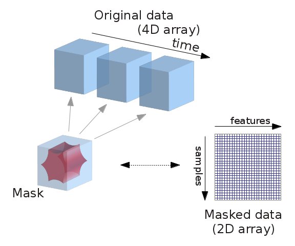
Fig. 1 Masking fMRI data.¶

Essentially, we can imagine overlaying a 3D grid on an image. Then, our mask tells us which cubes or “voxels” (like 3D pixels) to sample from. Since our Nifti images are 4D files, we can’t overlay a single grid – instead, we use a series of 3D grids (one for each volume in the 4D file), so we can get a measurement for each voxel at each timepoint.

Masker objects allow us to apply these masks! To start, we need to define a mask (or masks) that we’d like to apply. This could correspond to one or many regions of interest. Nilearn provides methods to define your own functional parcellation (using clustering algorithms such as k-means), and it also provides access to other atlases that have previously been defined by researchers.

Choosing regions of interest¶

In this tutorial, we’ll use the MSDL (multi-subject dictionary learning; [Varoquaux et al., 2011]) atlas, which defines a set of probabilistic ROIs across the brain.

import numpy as np

msdl_atlas = datasets.fetch_atlas_msdl()

msdl_coords = msdl_atlas.region_coords
n_regions = len(msdl_coords)

print(f'MSDL has {n_regions} ROIs, part of the following networks :\n{np.unique(msdl_atlas.networks)}.')

Nilearn ships with several atlases commonly used in the field, including the Schaefer atlas [Schaefer et al., 2017] and the Harvard-Oxford atlas.

It also provides us with easy ways to view these atlases directly. Because MSDL is a probabilistic atlas, we can view it using:

plotting.plot_prob_atlas(msdl_atlas.maps)

A quick side-note on the NiftiMasker zoo¶

We’d like to supply these ROIs to a Masker object. All Masker objects share the same basic structure and functionality, but each is designed to work with a different kind of ROI.

The canonical nilearn.input_data.NiftiMasker works well if we want to apply a single mask to the data, like a single region of interest.

But what if we actually have several ROIs that we’d like to apply to the data all at once? If these ROIs are non-overlapping, as in “hard” or deterministic parcellations, then we can use nilearn.input_data.NiftiLabelsMasker. Because we’re working with “soft” or probabilistic ROIs, we can instead supply these ROIs to nilearn.input_data.NiftiMapsMasker.

For a full list of the available Masker objects, see the Nilearn documentation.

Applying a Masker object¶

We can supply our MSDL atlas-defined ROIs to the NiftiMapsMasker object, along with resampling, filtering, and detrending parameters.

from nilearn import input_data

masker = input_data.NiftiMapsMasker(
    msdl_atlas.maps, resampling_target="data",
    t_r=2, detrend=True,
    low_pass=0.1, high_pass=0.01).fit()

One thing you might notice from the above code is that immediately after defining the masker object, we call the .fit method on it. This method may look familiar if you’ve previously worked with scikit-learn estimators!

You’ll note that we’re not supplying any data to this .fit method; that’s because we’re fitting the Masker to the provided ROIs, rather than to our data.

Dimensions, dimensions¶

We can now use this fitted masker to transform our data.

roi_time_series = masker.transform(development_dataset.func[0])
roi_time_series.shape

If you’ll remember, when we first looked at the data its original dimensions were (50, 59, 50, 168). Now, it has a shape of (168, 39). What happened?!

Rather than providing information on every voxel within our original 3D grid, we’re now only considering those voxels that fall in our 39 regions of interest provided by the MSDL atlas and aggregating across voxels within those ROIS. This reduces each 3D volume from a dimensionality of (50, 59, 50) to just 39, for our 39 provided ROIs.

You’ll also see that the “dimensions flipped;” that is, that we’ve transposed the matrix such that time is now the first rather than second dimension. This follows the scikit-learn convention that rows in a data matrix are samples, and columns in a data matrix are features.

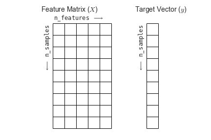
Fig. 2 The scikit-learn conventions for feature and target matrices. From Jake VanderPlas’s Python Data Science Handbook.¶

One of the nice things about working with nilearn is that it will impose this convention for you, so you don’t accidentally flip your dimensions when using a scikit-learn model!

Creating and viewing a connectome¶

The simplest and most commonly used kind of functional connectivity is pairwise correlation between ROIs. We can estimate it using nilearn.connectome.ConnectivityMeasure.

from nilearn.connectome import ConnectivityMeasure

correlation_measure = ConnectivityMeasure(kind='correlation')
correlation_matrix = correlation_measure.fit_transform([roi_time_series])[0]

We can then plot this functional connectivity matrix:

np.fill_diagonal(correlation_matrix, 0)
plotting.plot_matrix(correlation_matrix, labels=msdl_atlas.labels,
                     vmax=0.8, vmin=-0.8, colorbar=True)

Or view it as an embedded connectome:

plotting.view_connectome(correlation_matrix, edge_threshold=0.2,
                         node_coords=msdl_atlas.region_coords)

Accounting for noise sources¶

As we’ve already seen, maskers also allow us to perform other useful operations beyond just masking our data. One important processing step is correcting for measured signals of no interest (e.g., head motion). Our development_dataset also includes several of these signals of no interest that were generated during fMRIPrep pre-processing. We can access these with the confounds attribute, using development_dataset.confounds.

Let’s quickly check what these look like for our first participant:

import pandas as pd

pd.read_table(development_dataset.confounds[0]).head()

We can see that there are several different kinds of noise sources included! This is actually a subset of all possible fMRIPrep generated confounds that the Nilearn developers have pre-selected. We could access the full list by passing the argument reduce_confounds=False to our original call downloading the development_dataset. For most analyses, this list of confounds is reasonable, so we’ll use these Nilearn provided defaults. For your own analyses, make sure to check which confounds you’re using! For datasets processed with recent versions of fMRIPrep, check out the load_confounds functionality in Nilearn for a variety of confound processing strategies.

Importantly, we can pass these confounds directly to our masker object:

corrected_roi_time_series = masker.transform(
    development_dataset.func[0], confounds=development_dataset.confounds[0])
corrected_correlation_matrix = correlation_measure.fit_transform(
    [corrected_roi_time_series])[0]
np.fill_diagonal(corrected_correlation_matrix, 0)
plotting.plot_matrix(corrected_correlation_matrix, labels=msdl_atlas.labels,
                     vmax=0.8, vmin=-0.8, colorbar=True)

As before, we can also view this functional connectivity matrix as a connectome:

plotting.view_connectome(corrected_correlation_matrix, edge_threshold=0.2,
                         node_coords=msdl_atlas.region_coords)

In both the matrix and connectome forms, we can see a big difference when including the confounds! This is an important reminder to make sure that your data are cleaned of any possible sources of noise before running a machine learning analysis. Otherwise, you might be classifying participants on e.g. amount of head motion rather than a feature of interest!

1: Gael Varoquaux, Alexandre Gramfort, Fabian Pedregosa, Vincent Michel, and Bertrand Thirion. Multi-subject dictionary learning to segment an atlas of brain spontaneous activity. In Information Processing in Medical Imaging, 562–573. Springer Berlin Heidelberg, 2011.
2: Alexander Schaefer, Ru Kong, Evan M Gordon, Timothy O Laumann, Xi-Nian Zuo, Avram J Holmes, Simon B Eickhoff, and B T Thomas Yeo. Local-Global Parcellation of the Human Cerebral Cortex from Intrinsic Functional Connectivity MRI. Cerebral Cortex, 28(9):3095–3114, 07 2017. URL: https://doi.org/10.1093/cercor/bhx179, arXiv:https://academic.oup.com/cercor/article-pdf/28/9/3095/25696343/bhx179.pdf, doi:10.1093/cercor/bhx179.

COSN Nilearn

Extracting meaningful features

Contents