OHBM2021 Survey Feedback
This notebook contains code for rendering survey results from the OHBM 2021 Annual Meeting Evaluation. It is intended to accompany a recent OHBM Blog post exploring member feedback for the 2021 virtual event.
Note
All content is written in MyST and rendered using Jupyer Book. To ease navigation, several code cells are hidden by default. You can expand these code cells by clicking on the ‘Click to show’ buttons.
You can also load an interactive environment to further explore these data by clicking on the rocket icon in the upper right.
This will launch a new MyBinder session.
Right-clicking on the index.md file and selecting “Open in notebook editor” will allow you to re-analyze these data directly in the browser.
import numpy as np
import pandas as pd
from textwrap import wrap

import matplotlib.pyplot as plt
from matplotlib import cm
plt.rcParams.update({'font.size': 24})

import seaborn as sns

import warnings
warnings.filterwarnings('ignore')
We’ll use a limited subset of the full survey data. Data were collected on a Likert scale from 1-5, where 1 indicates ‘very poor’ experience with a given aspect of the annual meeting and 5 indicates an ‘excellent’ experience.
df = pd.read_csv('./ohbm2021-annual-meeting-eval.csv')
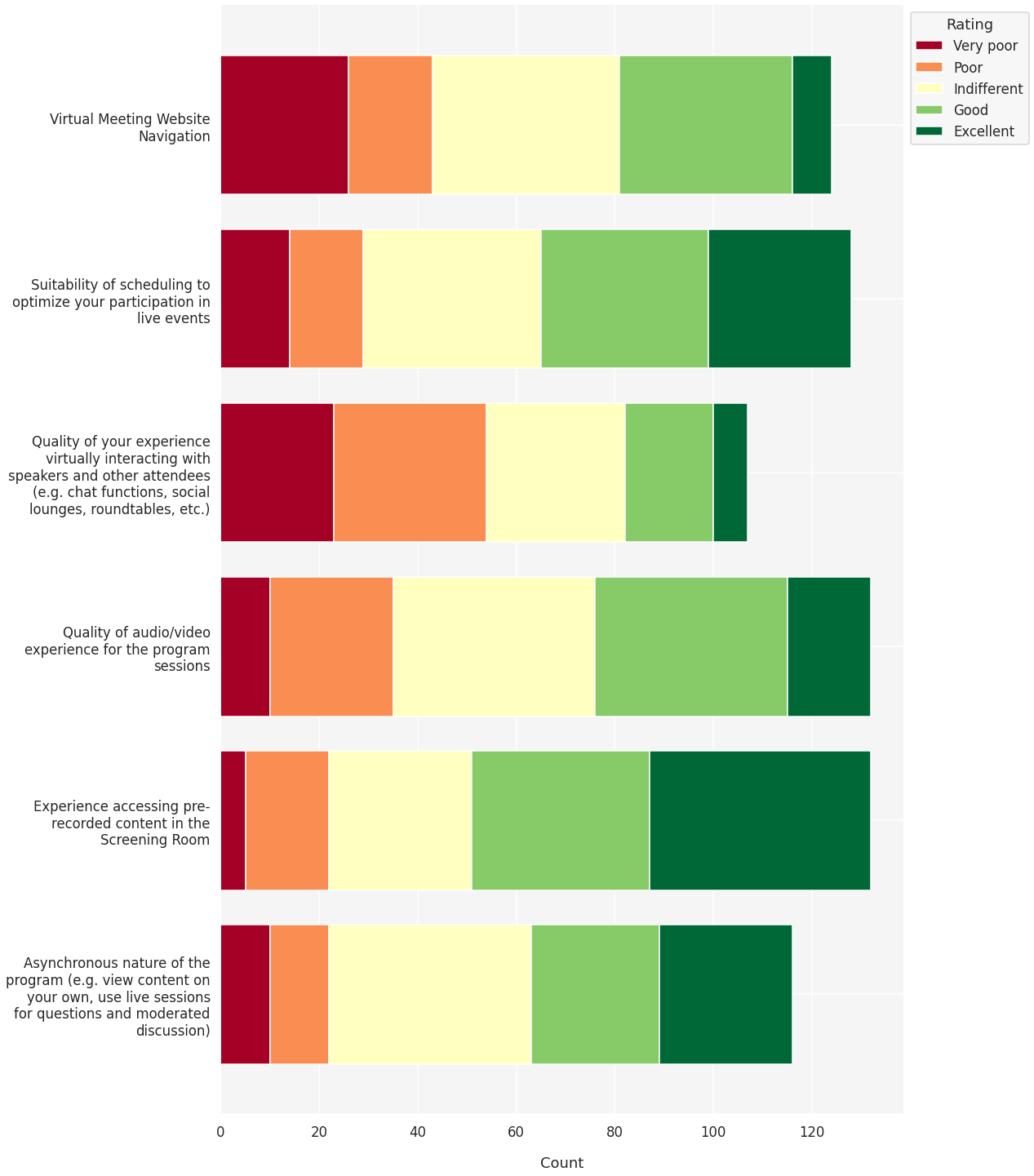
We’ll define a new function plot_stacked_bar to generate a stacked barplot showing the distribution of responses for each question.
We can then apply this function to the loaded pandas dataframe and plot the results.
def plot_stacked_bar(df, figwidth=25, textwrap=30):
    """
    A wrapper function to create a stacked bar plot.
    Seaborn does not implement this directly, so
    we'll use seaborn styling in matplotlib.

    Parameters
    ----------
    figwidth: float
        The desired width of the figure. Also controls
        spacing between bars.
    textwrap: int
        The number of characters (including spaces) allowed
        on a line before wrapping to a newline.
    """
    rdylgn = cm.get_cmap('RdYlGn', 5)
    colors = rdylgn(np.arange(rdylgn.N))
    reshape = pd.melt(df, var_name='option', value_name='rating')
    stack = reshape.rename_axis('count').reset_index().groupby(['option', 'rating']).count().reset_index()

    sns.set_style('darkgrid', {"axes.facecolor": "#F5F5F5"})
    sns.set_context('talk')
    fig, ax = plt.subplots(1, 1, figsize=(15, figwidth))
    bottom = np.zeros(len(stack['option'].unique()))
    labels = ['Very poor', 'Poor', 'Indifferent', 'Good', 'Excellent']

    for rating in range(1, 6):
        stackd = stack.query(f'rating == {rating}')
        ax.barh(y=stackd['option'], width=stackd['count'], left=bottom,
                tick_label=['\n'.join(wrap(s, textwrap)) for s in stackd['option']],
                color=colors[rating - 1], label=labels[rating - 1])
        bottom += np.asarray(stackd['count'])

    sns.despine()
    ax.set_xlabel('Count', labelpad=20)
    ax.legend(title='Rating', bbox_to_anchor=(1, 1))

    return ax
ax = plot_stacked_bar(df)
fig = ax.figure
fig.show()
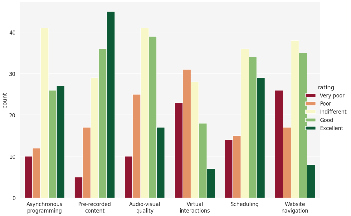
Alternatively, we can visualize this data with clustered bar charts,
showing the counts for each response to each question separately.
To do so, we’ll lightly modify our plot_stacked_bar and define a new plot_clustered_bar function.
We can then apply this function to the loaded pandas dataframe and plot the results.
def plot_clustered_bar(df, figwidth=20, textwrap=12):
    """
    A wrapper function to create a clustered bar plot.
    Styling kept as close as possible to `plot_stacked_bar`

    Parameters
    ----------
    figwidth: float
        The desired width of the figure. Also controls
        spacing between bars.
    textwrap: int
        The number of characters (including spaces) allowed
        on a line before wrapping to a newline.
    """
    rdylgn = cm.get_cmap('RdYlGn', 5)
    colors = rdylgn(np.arange(rdylgn.N))
    reshape = pd.melt(df, var_name='option', value_name='rating')
    stack = reshape.rename_axis('count').reset_index().groupby(['option', 'rating']).count().reset_index()

    labels = ['Very poor', 'Poor', 'Indifferent', 'Good', 'Excellent']
    questions = ['Asynchronous programming', 'Pre-recorded content',
                 'Audio-visual quality', 'Virtual interactions',
                 'Scheduling', 'Website navigation']

    sns.set(context='talk')
    sns.set_style('darkgrid', {"axes.facecolor": "#F5F5F5"})
    fig = sns.catplot(
        data=stack, kind="bar", x="option", y="count", hue="rating",
        hue_order=[1.0, 2.0, 3.0, 4.0, 5.0],
        ci="sd", palette=colors, legend=True, legend_out=True,
        height=10, aspect=figwidth/10)
    fig.despine()
    fig.set(xticks=range(len(df.columns)), xlabel='')
    fig.set_xticklabels(['\n'.join(wrap(q, textwrap)) for q in questions])
    for t, l in zip(fig._legend.texts, labels):
        t.set_text(l)

    return fig
fig = plot_clustered_bar(df)
fig;
We can see that ‘Experience accessing pre-recorded content in the Screening Room’ had the highest proportion of responses indicating an excellent experience, while ‘Virtual meeting website navigation’ and ‘Quality of your experience virtually interacting with speakers and other attendees’ had the highest number of respondents with a poor experience.
Rather than rely on visual comparisons, we can also directly quantify the proportion of ratings for each question:
proportion = []
questions = []
for c in df.columns:
    counts = df[c].value_counts(normalize=True).sort_index()
    proportion.append(counts.values * 100)
    questions.append(counts.name)

out = pd.DataFrame(data=proportion, index=questions,
                   columns=['1: Very poor', '2: Poor', '3: Indifferent',
                            '4: Good', '5: Excellent']).round(2)
out
| 1: Very poor | 2: Poor | 3: Indifferent | 4: Good | 5: Excellent | |
|---|---|---|---|---|---|
| Virtual Meeting Website Navigation | 20.97 | 13.71 | 30.65 | 28.23 | 6.45 |
| Suitability of scheduling to optimize your participation in live events | 10.94 | 11.72 | 28.12 | 26.56 | 22.66 |
| Quality of audio/video experience for the program sessions | 7.58 | 18.94 | 31.06 | 29.55 | 12.88 |
| Quality of your experience virtually interacting with speakers and other attendees (e.g. chat functions, social lounges, roundtables, etc.) | 21.50 | 28.97 | 26.17 | 16.82 | 6.54 |
| Experience accessing pre-recorded content in the Screening Room | 3.79 | 12.88 | 21.97 | 27.27 | 34.09 |
| Asynchronous nature of the program (e.g. view content on your own, use live sessions for questions and moderated discussion) | 8.62 | 10.34 | 35.34 | 22.41 | 23.28 |