An introduction to nilearn

An introduction to `nilearn`#

In this tutorial, we’ll see how the Python library nilearn allows us to easily perform machine learning and statistical learning analyses with neuroimaging data, specifically MRI and fMRI.

Note

You may notice that the name nilearn is reminiscent of scikit-learn, a popular Python library for machine learning. This is no accident! Nilearn and scikit-learn were created by overlapping teams, and nilearn is designed to bring machine LEARNing to NeuroImaging (NI) data.

Neuroimaging data#

While common machine learning pipelines assume tabular data, neuroimaging data does not have this structure. Instead, it has both spatial and temporal dependencies between successive data points. That is, knowing where and when something was measured tells you information about the surrounding data points.

We also know that neuroimaging data contains a lot of signal that’s not blood-oxygen-level dependent (BOLD), such as head motion. Since we don’t think that these other noise sources are related to neuronal firing, we often need to consider how we can make sure that our analyses are not driven by these noise sources.

These are all considerations that most machine learning software libraries are not designed to deal with! Nilearn therefore plays a crucial role in bringing machine learning concepts to the neuroimaging domain.

To get a sense of the problem, the quickest method is to just look at some data. You may have your own data locally that you’d like to work with. Nilearn also provides access to several neuroimaging data sets and atlases (we’ll talk about these a bit later).

These data sets (and atlases) are only accessible because research groups chose to make their collected data publicly available. We owe them a huge thank you for this! The data set we’ll use today was originally collected by Rebecca Saxe’s group at MIT and hosted on OpenNeuro.

The nilearn team preprocessed the data set with fMRIPrep and downsampled it to a lower resolution, so it’d be easier to work with. We can learn a lot about this data set directly from the Nilearn documentation. For example, we can see that this data set contains over 150 children and adults watching a short Pixar film. Let’s download the first 30 participants.

from nilearn import datasets

development_dataset = datasets.fetch_development_fmri(n_subjects=30)

Now, this development_dataset object has several attributes which provide access to the relevant information. For example, development_dataset.phenotypic provides access to information about the participants, such as whether they were children or adults. We can use development_dataset.func to access the functional MRI (fMRI) data.

Let’s use the nibabel library to learn a little bit about this data:

import nibabel as nib

img = nib.load(development_dataset.func[0])
img.shape

(50, 59, 50, 168)

This means that there are 168 volumes, each with a 3D structure of (50, 59, 50).

Getting into the data: subsetting and viewing#

Nilearn also provides many methods for plotting this kind of data. For example, we can use nilearn.plotting.view_img to launch at interactive viewer. Because each fMRI run is a 4D time series (three spatial dimensions plus time), we’ll also need to subset the data when we plot it, so that we can look at a single 3D image. Nilearn provides (at least) two ways to do this: with nilearn.image.index_img, which allows us to index a particular frame–or several frames–of a time series, and nilearn.image.mean_img, which allows us to take the mean 3D image over time.

Putting these together, we can interatively view the mean image of the first participant using:

import matplotlib.pyplot as plt
from nilearn import image
from nilearn import plotting

mean_image = image.mean_img(development_dataset.func[0])
plotting.view_img(mean_image, threshold=None)

Extracting signal from fMRI volumes#

As you can see, this data is decidedly not tabular! What we’d like is to extract and transform meaningful features from this data, and store it in a format that we can easily work with. Importantly, we could work with the full time series directly. But we often want to reduce the dimensionality of our data in a structured way. That is, we may only want to consider signal within certain learned or pre-defined regions of interest (ROIs), and when taking into account known sources of noise. To do this, we’ll use nilearn’s Masker objects. What are the masker objects ? First, let’s think about what masking fMRI data is doing:

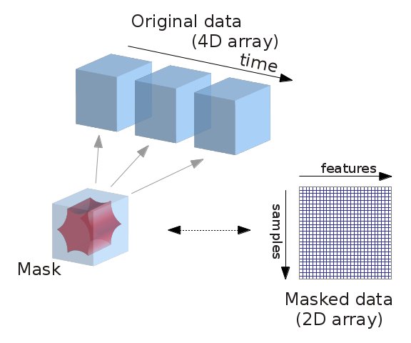
_images/masking.jpg — Fig. 1 Masking fMRI data.#

Essentially, we can imagine overlaying a 3D grid on an image. Then, our mask tells us which cubes or “voxels” (like 3D pixels) to sample from. Since our Nifti images are 4D files, we can’t overlay a single grid – instead, we use a series of 3D grids (one for each volume in the 4D file), so we can get a measurement for each voxel at each timepoint.

Masker objects allow us to apply these masks! To start, we need to define a mask (or masks) that we’d like to apply. This could correspond to one or many regions of interest. Nilearn provides methods to define your own functional parcellation (using clustering algorithms such as k-means), and it also provides access to other atlases that have previously been defined by researchers.

Choosing regions of interest#

In this tutorial, we’ll use the MSDL (multi-subject dictionary learning; [1]) atlas, which defines a set of probabilistic ROIs across the brain.

import numpy as np

msdl_atlas = datasets.fetch_atlas_msdl()

msdl_coords = msdl_atlas.region_coords
n_regions = len(msdl_coords)

print(f'MSDL has {n_regions} ROIs, part of the following networks :\n{np.unique(msdl_atlas.networks)}.')

[fetch_atlas_msdl] Dataset found in /Users/emdupre/nilearn_data/msdl_atlas
MSDL has 39 ROIs, part of the following networks :
['Ant IPS' 'Aud' 'Basal' 'Cereb' 'Cing-Ins' 'D Att' 'DMN' 'Dors PCC'
 'L V Att' 'Language' 'Motor' 'Occ post' 'R V Att' 'Salience' 'Striate'
 'Temporal' 'Vis Sec'].

Nilearn ships with several atlases commonly used in the field, including the Schaefer atlas and the Harvard-Oxford atlas.

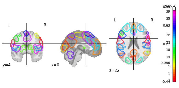
It also provides us with easy ways to view these atlases directly. Because MSDL is a probabilistic atlas, we can view it using:

plotting.plot_prob_atlas(msdl_atlas.maps)

<nilearn.plotting.displays._slicers.OrthoSlicer at 0x17f9bfc40>

_images/0e4f3a59398d55683fb344d60f003633b67e30f160b4310c82656b89ee622953.png

A quick side-note on the NiftiMasker zoo#

We’d like to supply these ROIs to a Masker object. All Masker objects share the same basic structure and functionality, but each is designed to work with a different kind of ROI.

The canonical nilearn.maskers.NiftiMasker works well if we want to apply a single mask to the data, like a single region of interest.

But what if we actually have several ROIs that we’d like to apply to the data all at once? If these ROIs are non-overlapping, as in “hard” or deterministic parcellations, then we can use nilearn.maskers.NiftiLabelsMasker. Because we’re working with “soft” or probabilistic ROIs, we can instead supply these ROIs to nilearn.maskers.NiftiMapsMasker.

For a full list of the available Masker objects, see the Nilearn documentation.

Applying a Masker object#

We can supply our MSDL atlas-defined ROIs to the NiftiMapsMasker object, along with resampling, filtering, and detrending parameters.

from nilearn import maskers

masker = maskers.NiftiMapsMasker(
    msdl_atlas.maps, resampling_target="data",
    t_r=2, detrend=True,
    low_pass=0.1, high_pass=0.01).fit()

One thing you might notice from the above code is that immediately after defining the masker object, we call the .fit method on it. This method may look familiar if you’ve previously worked with scikit-learn estimators!

You’ll note that we’re not supplying any data to this .fit method; that’s because we’re fitting the Masker to the provided ROIs, rather than to our data.

Dimensions, dimensions#

We can use this fitted masker to transform our data.

roi_time_series = masker.transform(development_dataset.func[0])
roi_time_series.shape

(168, 39)

If you’ll remember, when we first looked at the data its original dimensions were (50, 59, 50, 168). Now, it has a shape of (168, 39). What happened?!

Rather than providing information on every voxel within our original 3D grid, we’re now only considering those voxels that fall in our 39 regions of interest provided by the MSDL atlas and aggregating across voxels within those ROIS. This reduces each 3D volume from a dimensionality of (50, 59, 50) to just 39, for our 39 provided ROIs.

You’ll also see that the “dimensions flipped;” that is, that we’ve transposed the matrix such that time is now the first rather than second dimension. This follows the scikit-learn convention that rows in a data matrix are samples, and columns in a data matrix are features.

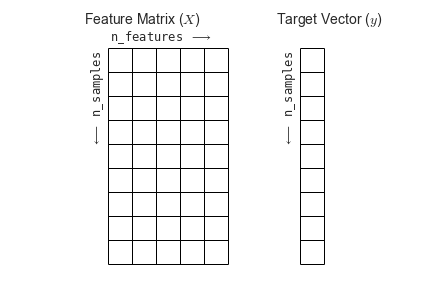
_images/samples-features.png — Fig. 2 The scikit-learn conventions for feature and target matrices. From Jake VanderPlas’s *Python Data Science Handbook*.#

One of the nice things about working with nilearn is that it will impose this convention for you, so you don’t accidentally flip your dimensions when using a scikit-learn model!

Creating and viewing a connectome#

The simplest and most commonly used kind of functional connectivity is pairwise correlation between ROIs. We can estimate it using nilearn.connectome.ConnectivityMeasure.

from nilearn.connectome import ConnectivityMeasure

correlation_measure = ConnectivityMeasure(kind='correlation')
correlation_matrix = correlation_measure.fit_transform([roi_time_series])[0]

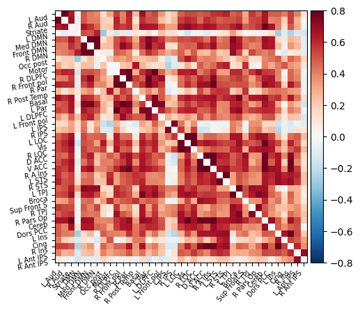
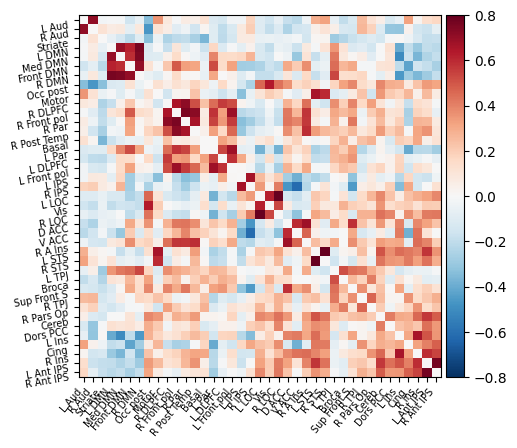
We can then plot this functional connectivity matrix:

np.fill_diagonal(correlation_matrix, 0)
plotting.plot_matrix(correlation_matrix, labels=msdl_atlas.labels,
                     vmax=0.8, vmin=-0.8, colorbar=True)

<matplotlib.image.AxesImage at 0x17ffdd7c0>

_images/1cc3c97afa05a888d6e55d2683c0e6cbee7f80e09aa0c01226c1d50c199b9d21.png

Or view it as an embedded connectome:

plotting.view_connectome(correlation_matrix, edge_threshold=0.2,
                         node_coords=msdl_atlas.region_coords)

Accounting for noise sources#

As we’ve already seen, maskers also allow us to perform other useful operations beyond just masking our data. One important processing step is correcting for measured signals of no interest (e.g., head motion). Our development_dataset also includes several of these signals of no interest that were generated during fMRIPrep pre-processing. We can access these with the confounds attribute, using development_dataset.confounds.

Let’s quickly check what these look like for our first participant:

import pandas as pd

pd.read_table(development_dataset.confounds[0]).head()

	trans_x	trans_y	trans_z	rot_x	rot_y	framewise_displacement	a_comp_cor_00	a_comp_cor_01	a_comp_cor_02	a_comp_cor_03	a_comp_cor_04	a_comp_cor_05	csf	white_matter
0	0.000000	0.000000	0.000000	0.000000	-0.000000	0.000000	0.000000	0.000000	0.000000	0.000000	0.000000	0.000000	525.521464	473.476960
1	0.002290	0.039488	-0.000004	0.000000	0.000190	0.051301	-0.009419	0.064324	-0.046474	0.006744	-0.007179	0.025285	529.577966	476.734232
2	-0.000011	-0.104030	-0.009560	0.000164	0.000366	0.172322	-0.013124	0.010970	0.072557	0.030795	0.015773	-0.063280	531.250261	476.517911
3	-0.000031	0.169104	0.013041	-0.000843	0.000453	0.350465	0.033150	0.025784	0.036211	0.005530	0.048968	-0.025824	531.240585	476.460569
4	-0.000061	-0.145348	-0.025025	0.000060	0.000386	0.401084	-0.035600	-0.035397	-0.127860	0.001092	-0.031902	0.048258	531.931781	476.174483

We can see that there are several different kinds of noise sources included! This is actually a subset of all possible fMRIPrep generated confounds that the Nilearn developers have pre-selected. We could access the full list by passing the argument reduce_confounds=False to our original call downloading the development_dataset. For most analyses, this list of confounds is reasonable, so we’ll use these Nilearn provided defaults. For your own analyses, make sure to check which confounds you’re using!

Importantly, we can pass these confounds directly to our masker object:

corrected_roi_time_series = masker.transform(
    development_dataset.func[0], confounds=development_dataset.confounds[0])
corrected_correlation_matrix = correlation_measure.fit_transform(
    [corrected_roi_time_series])[0]
np.fill_diagonal(corrected_correlation_matrix, 0)
plotting.plot_matrix(corrected_correlation_matrix, labels=msdl_atlas.labels,
                     vmax=0.8, vmin=-0.8, colorbar=True)

<matplotlib.image.AxesImage at 0x317ead310>

_images/73ab92ab3b3227fa16d6bf2a4976e18dc93206cdf5eb890995f46ded57159010.png

As before, we can also view this functional connectivity matrix as a connectome:

plotting.view_connectome(corrected_correlation_matrix, edge_threshold=0.2,
                         node_coords=msdl_atlas.region_coords)

In both the matrix and connectome forms, we can see a big difference when including the confounds! This is an important reminder to make sure that your data are cleaned of any possible sources of noise before running a machine learning analysis. Otherwise, you might be classifying participants on e.g. amount of head motion rather than a feature of interest!

1: Gaël Varoquaux, Alexandre Gramfort, Fabian Pedregosa, Vincent Michel, and Bertrand Thirion. Multi-subject dictionary learning to segment an atlas of brain spontaneous activity. In Information Processing in Medical Imaging, 562–573. Springer Berlin Heidelberg, 2011.